Introduction
A modern CPU runs at billions of clock cycles per second. It can execute programs, manage an operating system, and handle many different tasks at once. So why do AI systems often need GPUs and specialized accelerators?
The answer is not simply that CPUs are too slow.
AI workloads place unusual demands on a computer. They involve large amounts of repeated arithmetic, enormous collections of numerical data, and frequent movement of that data between memory and processing units. Increasing clock speed addresses only part of the problem.
To understand AI hardware, we need to look at three things together: how calculations are performed, how many can happen in parallel, and how efficiently data reaches the hardware.
We can begin with something much simpler than a language model: logic gates.
Chapter 1: From Logic Gates to Arithmetic
Logic gates operate on binary signals. An AND gate, an OR gate, and a NOT gate perform simple logical operations, but combinations of gates can implement arithmetic.
A half adder adds two bits. A full adder also handles an incoming carry. Connecting these circuits allows a processor to add larger binary numbers.
Multiplication requires more circuitry. One basic method forms partial products and adds them together. Real processors use optimized designs, but the underlying principle remains: arithmetic is performed by carefully arranged digital circuits.
Now imagine a calculation that repeatedly multiplies two values and adds the product to a running total:
Running total ← Running total + A × B
This is called a multiply-accumulate operation, often abbreviated MAC. It appears throughout neural-network computation.
If a processor has limited arithmetic hardware, it must spread a large collection of these operations across many execution steps. Adding more arithmetic units can allow more work to happen in parallel, provided the operations are independent and data arrives quickly enough.
AI accelerators build on the same digital foundations as other processors. Their advantage comes from how they organize arithmetic circuits, storage, and data movement around particular workloads.
Chapter 2: Why Clock Speed Does Not Tell the Whole Story
A CPU running at 4 GHz has four billion clock cycles per second. That does not mean it completes exactly four billion instructions, multiplications, or AI operations every second.
Some instructions require multiple cycles. Modern processors can also issue several instructions in a cycle, overlap their execution, and operate on multiple data elements with a single instruction.
Performance therefore depends on the amount of useful work completed per cycle as well as the number of cycles per second.
Consider two imaginary processors. One runs at a higher clock speed but has only a few arithmetic units available for a particular operation. The other runs at a lower clock speed but can perform many more of those operations simultaneously. For a sufficiently parallel workload, the second processor may finish sooner.
General-purpose CPUs devote substantial resources to handling varied and unpredictable programs. Branch prediction, caches, instruction scheduling, and low-latency execution help them respond well to many different tasks.
AI accelerators place more emphasis on repeated numerical operations. They trade some general-purpose flexibility for greater throughput or energy efficiency on supported calculations.
CPUs can run AI models, and they may be entirely adequate for smaller workloads. Specialized hardware becomes valuable when the required throughput, response time, or power efficiency exceeds what a particular CPU system can provide.
Chapter 3: The Repeated Calculation Inside Neural Networks
Many neural-network layers combine input values with learned weights.
A simple example uses three input values:
Inputs: [1, 2, 3]
And three weights:
Weights: [4, 5, 6]
Multiplying matching values and adding the products gives:
1 × 4 + 2 × 5 + 3 × 6 = 32
This calculation is a dot product.
One output value is manageable. A neural-network layer may need thousands of outputs, each calculated using a different collection of weights. Processing multiple inputs increases the work further.
These calculations can be organized as matrix multiplication. A matrix is a rectangular arrangement of numbers, and each output element is formed by combining a row from one matrix with a column from another.
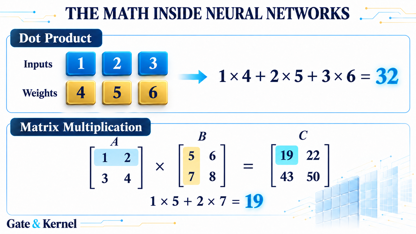
For a small example, suppose matrix A has the rows [1, 2] and [3, 4], while matrix B has the rows [5, 6] and [7, 8]. The first output element is:
1 × 5 + 2 × 7 = 19
The remaining output elements are 22, 43, and 50.
Larger matrices repeat the same basic pattern at much greater scale. If A has M rows and K columns, and B has K rows and N columns, their product contains M × N output values. A conventional dense implementation requires M × N × K multiply-accumulate steps.
This repeated structure creates opportunities for specialized hardware.
Chapter 4: From Individual Values to Vectors and Matrices
A scalar operation works on individual values. A vector operation applies an operation across multiple elements. A matrix operation combines rows and columns to produce a collection of accumulated results.
Modern CPUs already support vector processing. They do not necessarily process every number individually. Vector instructions can perform useful work on several elements at once, making them important for scientific computing, multimedia, and AI.
Matrix hardware goes further by organizing execution around repeated combinations of operands.
Imagine that one input value contributes to several output elements. Instead of repeatedly fetching it for separate operations, hardware can retain it locally and distribute it to multiple arithmetic units.
Likewise, partial results can remain close to the circuits updating them. The hardware may perform many multiply-accumulate steps before writing the completed results elsewhere.
A tile is a small block of a larger matrix. Software and hardware often divide a large multiplication into tiles that fit available storage and execution resources.
The benefit comes from both parallel computation and reuse. Matrix acceleration is effective when its organization matches the shapes and numerical formats of the workload.
A large matrix engine can still be inefficient when given a very narrow or unusually shaped operation. Having more arithmetic units helps only when enough useful work reaches them.
Chapter 5: Fast Arithmetic Still Has to Wait for Data
Before an arithmetic unit can multiply two numbers, those numbers must be available.
A processor accesses data through a hierarchy of storage, including registers, caches, and main memory. Accelerators also use local storage and their own memory systems. These levels differ in capacity, bandwidth, latency, and energy cost.
Memory capacity describes how much data can be stored. Memory bandwidth describes how much data can be transferred per second. A system may have enough capacity to hold a model while lacking the bandwidth to process it quickly.
Consider an illustrative eight-billion-parameter model stored at two bytes per parameter:
8 billion × 2 bytes = 16 GB of weight data
That excludes working buffers, cached attention information, and other overhead.
If an execution step had to stream those 16 GB through a memory interface sustaining 100 GB per second, the transfer alone would take approximately:
16 GB ÷ 100 GB/s = 0.16 seconds
This is a simplified bandwidth example, not a prediction for a particular model or computer. Caching, compression, batching, architecture, and software change the actual traffic.
Nevertheless, the principle is clear: making multiplication faster cannot eliminate time spent waiting for operands.
Performance analysis distinguishes compute-limited operations from memory-limited operations. Which limit dominates depends partly on arithmetic intensity: the amount of computation performed per byte transferred at the memory level being examined.
Chapter 6: Why Reusing Data Is So Important
Suppose a weight is fetched from memory and used once. Its transfer cost supports only a small amount of computation.
Now suppose that same weight is fetched once, retained locally, and used for many input values. The transfer supports much more useful work.
This is why matrix shape and batching matter.
A matrix-vector operation combines a matrix with a single vector. A matrix-matrix operation can apply the same matrix to several vectors together, creating opportunities to reuse its values.
For example, processing one input at a time may require repeatedly reading the same weights. Processing a group of inputs together can allow the hardware to reuse those weights while calculating multiple results.
This does not mean that larger batches are always better. They require additional storage, and waiting to assemble a batch can affect response latency.
Tiling provides another form of reuse. A small group of input values and weights is brought into fast storage, used for several calculations, and then replaced with the next group.
NVIDIA’s matrix-multiplication documentation describes how dimensions and arithmetic intensity affect whether an operation is limited by computation or data transfer. The broader principle applies beyond any single GPU: hardware utilization depends on the work’s organization, not just its operation count.
Chapter 7: Why a Chatbot Reads and Writes Differently
A typical autoregressive language model processes a request in two major phases: prefill and decode.
During prefill, it processes the input prompt. Many token positions can be handled in parallel within a layer, creating opportunities for larger matrix operations. The model also builds information used by subsequent attention calculations.
During decode, it generates additional tokens step by step. A token may represent a word, part of a word, punctuation, or another text fragment.
In conventional generation, the next step depends on the token selected in the previous step.
This limits how much future output can be generated independently for one sequence.
As a simplified example, a linear layer processing 256 prompt positions might multiply a 256-by-K input matrix by a K-by-N weight matrix.
Processing one new position during decode might instead multiply a 1-by-K input by those weights.
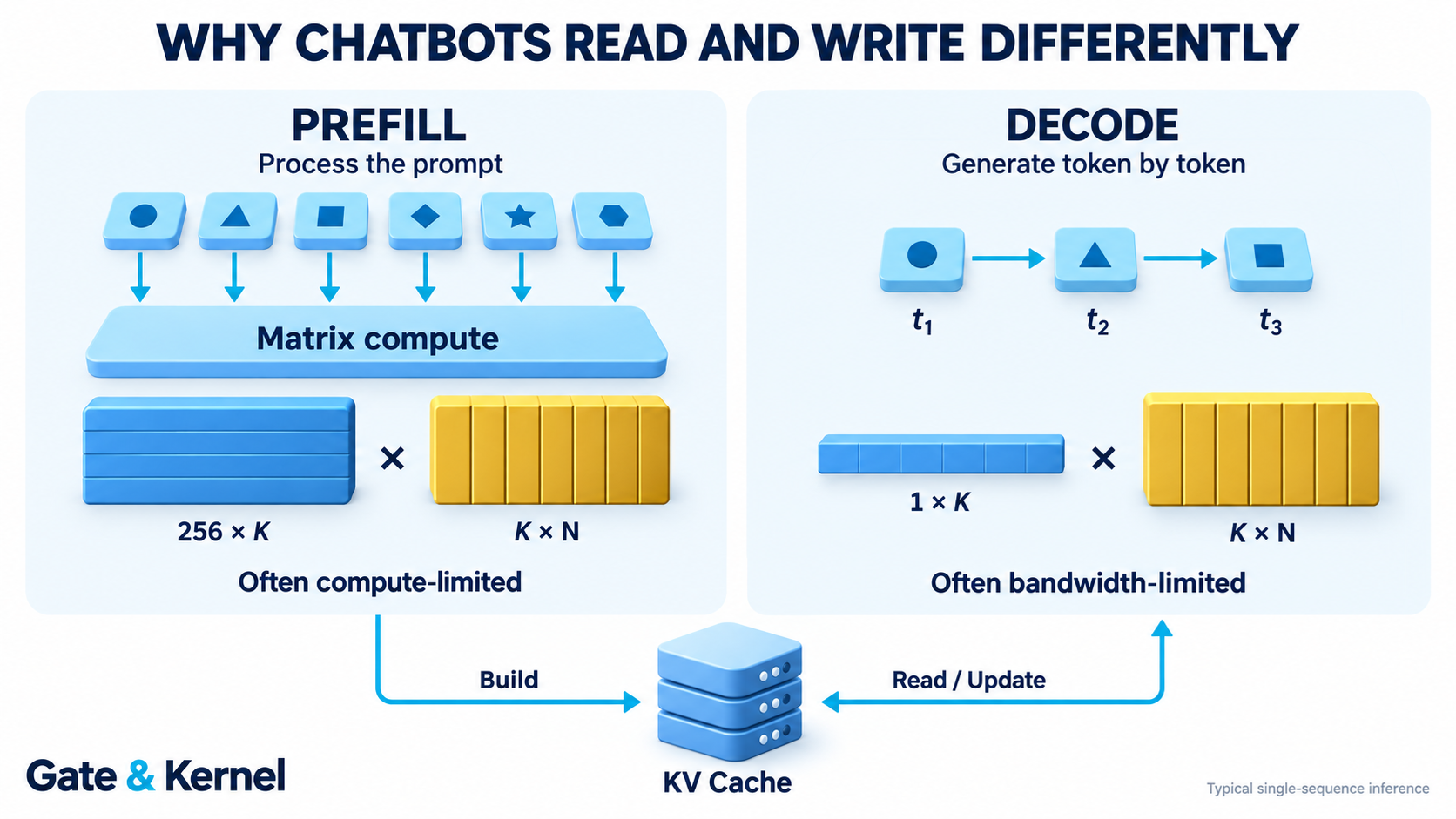
The second operation provides less opportunity to reuse weights across input rows.
Consequently, prefill often benefits strongly from matrix compute throughput, while single-sequence decode frequently encounters memory-bandwidth limits. The exact bottleneck depends on the model, context length, batch size, and implementation.
Language models commonly maintain a key-value cache, or KV cache, to avoid recalculating earlier attention keys and values. This saves computation but consumes memory and requires data access.
Serving multiple sequences together can improve hardware utilization, although the system must also accommodate their caches and latency requirements. This helps explain why a computer that processes a prompt quickly may still generate its answer relatively slowly.
Chapter 8: Smaller Numbers Can Mean Less Work
AI hardware also improves efficiency by using numerical formats suited to the model.
A 32-bit floating-point value occupies four bytes. A 16-bit value occupies two bytes. An 8-bit value occupies one byte.
For one million values, the raw storage is approximately 4 MB, 2 MB, or 1 MB respectively. Smaller representations can reduce both storage requirements and memory traffic.
Supported lower-precision arithmetic may also use less circuit area or energy, allowing hardware to provide more operations within a given budget.
However, fewer bits mean fewer representable values. Choosing a format requires a trade-off between efficiency and numerical behavior.
FP16 and BF16 both use 16 bits, but allocate them differently. BF16 provides a broad exponent range with less fraction precision. FP8 offers further reductions, with different formats making different range-and-precision trade-offs.
A common approach multiplies lower-precision inputs while accumulating results in a wider format. For example, supported hardware can multiply FP8 inputs and accumulate into FP32. NVIDIA documents this capability for its Hopper architecture.
Quantization maps values into a reduced representation. Its usefulness depends on the model, scaling method, software, and hardware support. Smaller formats can improve efficiency, but acceptable output quality must be checked rather than assumed.
Chapter 9: Where RISC-V Fits into AI Acceleration
RISC-V is an instruction set architecture: a definition of operations software can request and the behavior those operations must provide.
It is not a single processor design. Different RISC-V implementations can have very different performance, memory systems, and execution hardware.
Its standard vector extension, RVV, provides a foundation for data-parallel computation. Vector processing remains useful for many AI operations beyond matrix multiplication, including normalization, activation functions, reductions, and conversion between numerical formats.
Matrix-extension work explores several ways to build on or complement that foundation.
Batched dot products reuse vector operands to calculate several accumulated results.
Integrated Matrix Extensions, or IME, keep matrix operands and results in the vector-register model.
Vector Matrix Extensions, or VME, use vector-register inputs with dedicated matrix accumulator state.
Attached Matrix Extensions, or AME, provide a more separate organization for matrix operands and results.
These approaches differ primarily in where data lives and how computation accesses it. They illustrate the same architectural choices discussed throughout this article: parallel arithmetic, local accumulation, and efficient movement of operands. RISC-V International describes the three matrix approaches as complementary directions under development.
As of this article’s October 15, 2026 review, readers should distinguish established RVV support from evolving matrix proposals and vendor-specific implementations. An extension mentioned in a presentation is not automatically available on every RISC-V processor.
Chapter 10: The Whole System Determines AI Performance
Even excellent matrix hardware cannot accelerate every part of a program.
A neural network also performs operations such as normalization, activation, indexing, and data conversion. The surrounding application prepares inputs, schedules work, manages memory, and delivers outputs.
Suppose matrix multiplication accounts for 80% of execution time. Making it ten times faster leaves:
20% + 80% ÷ 10 = 28% of the original execution time
The whole program becomes approximately 3.6 times faster. The remaining work limits the overall improvement.
Software determines how effectively hardware is used. Optimized libraries select suitable kernels, arrange data, and schedule operations. Some optimizations combine operations so that intermediate results do not have to be repeatedly written to and read from slower memory.
The CPU remains valuable for general-purpose execution and coordination. Depending on the system, it may also perform part or all of the model’s numerical computation.
Meaningful evaluation therefore considers more than clock speed or peak operations per second. For an interactive language model, useful measurements include time to first token, output-token latency, memory consumption, and performance at the required output quality.
The best design is the one that meets the application’s requirements as a complete system.
Conclusion
AI hardware begins with the same foundations as other digital computing: logic gates, arithmetic circuits, registers, and memory.
What changes is how those components are organized.
A fast CPU can execute a wide variety of programs, but demanding AI workloads also benefit from extensive parallel arithmetic, efficient matrix operations, suitable numerical formats, and repeated reuse of data close to the execution units.
GPUs, specialized accelerators, and emerging RISC-V matrix extensions explore different ways to provide those capabilities.
The crucial question is not simply how fast a processor’s clock runs. It is how much useful work the system can perform, how quickly it can supply the required data, and how much energy the complete process consumes.
That is why AI needs more than a fast CPU.